Project 5: Image Generation and Manipulation with Diffusion Models

Part 0: Testing Images

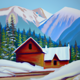
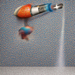
We procured images just to test how things work.

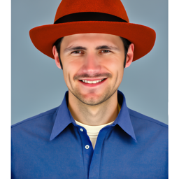
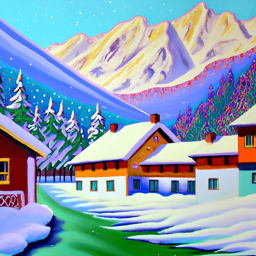
All these images were produced using a seed of 356. We experimented with different inference steps.

Part 1.1: Implementing the Forward Process

A key part of diffusion is the forward process, which takes a clean image and adds noise to it. In this part, we implemented this process using the following equations:

q(x_t | x₀) = N(x_t ; √(ᾱ_t) x₀, (1 - ᾱ_t) I)

x_t = √(ᾱ_t) x₀ + √(1 - ᾱ_t) ε, where ε ~ N(0, 1)

Given a clean image x₀, we get a noisy image x_t at timestep t by sampling from a Gaussian with mean √(ᾱ_t) x₀ and variance (1 - ᾱ_t). Note that the forward process not only adds noise but also scales the image.

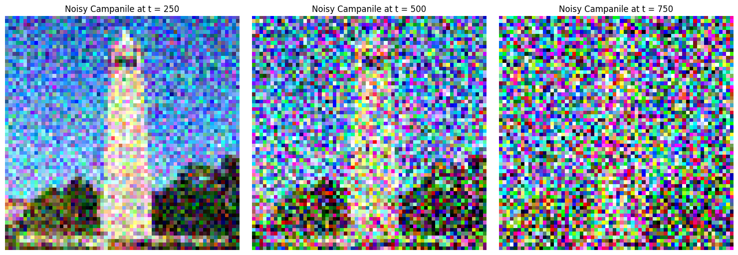
We used the alphas_cumprod variable, which contains the ᾱ_t for all t ∈ [0, 999]. Since t = 0 corresponds to a clean image and larger t corresponds to more noise, ᾱ_t is close to 1 for small t and close to 0 for large t.

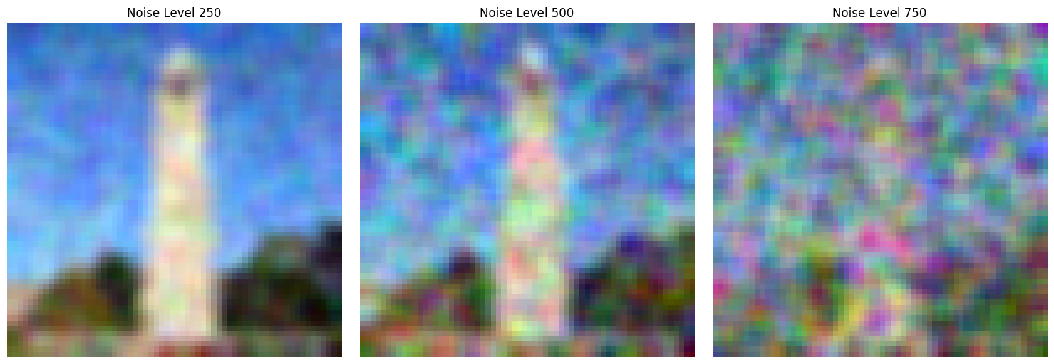
We ran the forward process on the test image with t ∈ [250, 500, 750]. Below are the results, showing progressively noisier images.

Noise Levels at Different Timesteps — Noise levels at timesteps 250, 500, and 750.

Part 1.2: Naively Denoising with Gaussian Blur

We attempted to naively smooth out the noise by applying a Gaussian blur to the noisy images.

Gaussian Blurred Images — Images after applying Gaussian blur.

Part 1.3: Denoising with a Pretrained Diffusion Model

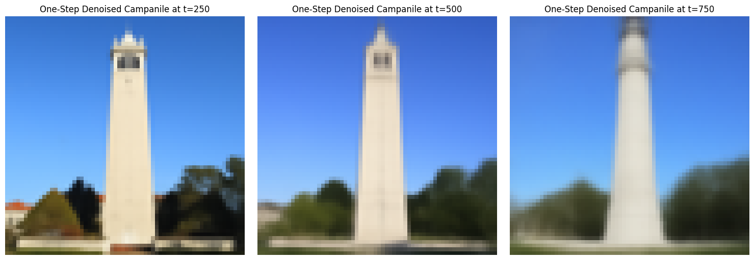
We used a pretrained diffusion model to denoise the images. The UNet model stage_1.unet has been trained on a large dataset of (x₀, x_t) pairs of images. It can recover Gaussian noise from the image, allowing us to estimate the original image by effectively reversing the noise addition process.

Denoised Image with UNet — Denoised image using the pretrained UNet model.

Part 1.4: Iterative Denoising

While the UNet model performs well, it struggles with images that have higher noise levels. To improve the results, we implemented an iterative denoising process using the following equation:

x_t' = [√(ᾱ_t') β_t / (1 - ᾱ_t)] x₀ + [√(α_t)(1 - ᾱ_t') / (1 - ᾱ_t)] x_t + v_σ

Where:

x_t is the image at timestep t
x_t' is the image at timestep t' (less noisy, t' < t)
α_t = ᾱ_t / ᾱ_t'
β_t = 1 - α_t
x₀ is our current estimate of the clean image

This process allows us to skip steps and denoise more efficiently.

Iterative Denoising Results — Result after 5 iterative denoising steps.

Comparison of Denoising Methods — Comparison between one-step and iterative denoising.

Part 1.5 and 1.6: Generating Images from Scratch and Classifier-Free Guidance

Using the iterative_denoise function, we generated images from scratch by starting with random noise and setting i_start = 0. This allows the model to create images based on the text prompt "a high quality photo."

We implemented Classifier-Free Guidance (CFG) to enhance image quality. In CFG, we compute both a noise estimate conditioned on a text prompt (ε_c) and an unconditional noise estimate (ε_u). We then compute:

ε = ε_u + γ (ε_c - ε_u)

Where γ controls the strength of CFG. Setting γ > 1 leads to higher quality images by amplifying the effect of the conditioning prompt.

Generated Images without CFG — Images generated without CFG.

Generated Images with CFG — Images generated with CFG (γ > 1).

Part 1.7: Image Editing with Diffusion Models

We explored how adding noise to a real image and then denoising it can effectively edit the image. The more noise we add, the more significant the edits. This works because the denoising process forces the noisy image back onto the manifold of natural images, allowing the model to "hallucinate" new content.

Part 1.7.1: Applying Edits to Web and Hand-Drawn Images

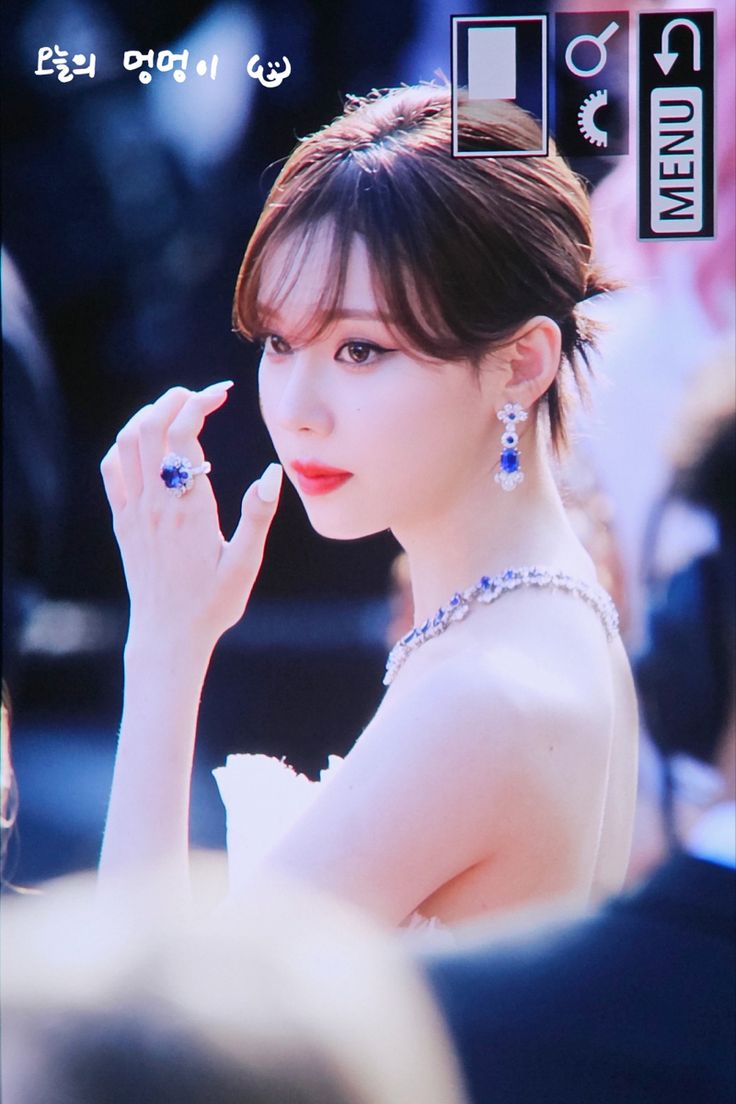
We applied these editing techniques to images downloaded from the web and hand-drawn images.

Web Image:

Hand-Drawn Images:

Part 1.7.2: Inpainting with Diffusion Models

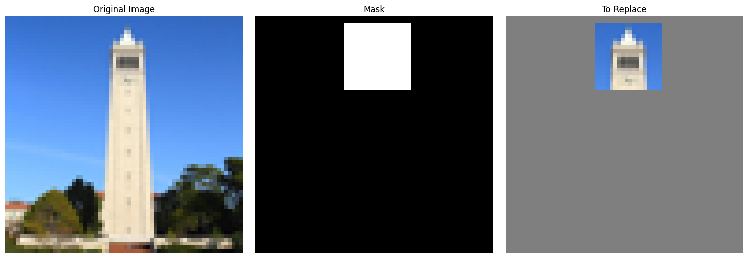
We implemented inpainting using the RePaint approach. Given an image x_orig and a binary mask m, we created a new image that preserves the original content where m = 0 and generates new content where m = 1. At each denoising step, we updated x_t as:

x_t ← m x_t + (1 - m) forward(x_orig, t)

This ensures that regions outside the mask remain unchanged while the model inpaints the masked areas.

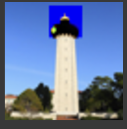
Inpainting Mask — Mask used for inpainting.

Inpainting Result — Result after inpainting.

Part 1.7.3: Text-Conditioned Image-to-Image Translation

We performed image-to-image translation guided by text prompts. By changing the prompt from "a high quality photo" to specific descriptions, we manipulated the image content in a controlled manner.

Ship to Campanile — Transformation from ship to campanile.

Village to Snowman — Transformation from village to snowman.

Dog to Winter Scene — Transformation from dog to winter scene.

Part 1.8: Creating Visual Anagrams

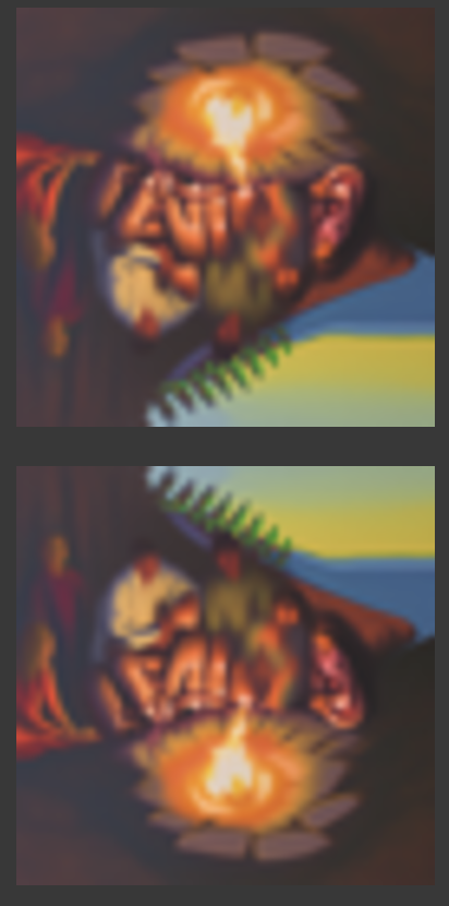
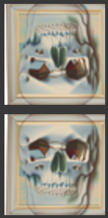
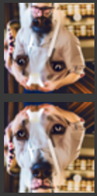
We implemented Visual Anagrams to create optical illusions with diffusion models. For example, we created an image that looks like "an oil painting of an old man," but when flipped upside down reveals "an oil painting of people around a campfire."

We achieved this by denoising an image x_t with two different prompts, flipping one of the noise estimates, and averaging them:

ε₁ = UNet(x_t, t, p₁)

ε₂ = flip(UNet(flip(x_t), t, p₂))

ε = (ε₁ + ε₂) / 2

Old Man / Campfire — "An oil painting of an old man" / "people around a campfire"

Skull / Village — "A skull" / "a village landscape"

Part 1.9: Creating Hybrid Images with Factorized Diffusion

We implemented Factorized Diffusion to create hybrid images, combining elements from two different prompts. We merged low frequencies from one noise estimate with high frequencies from another:

ε₁ = UNet(x_t, t, p₁)

ε₂ = UNet(x_t, t, p₂)

ε = lowpass(ε₁) + highpass(ε₂)

Dog / Man Hybrid — Hybrid of "a dog" and "a man."

Rocket / Fire Hybrid — Hybrid of "a rocket ship" and "fire."

Skull / Waterfall Hybrid — Hybrid of "a skull" and "a waterfall."

Project 5B

Part 1: Training a Single-Step Denoising U-Net

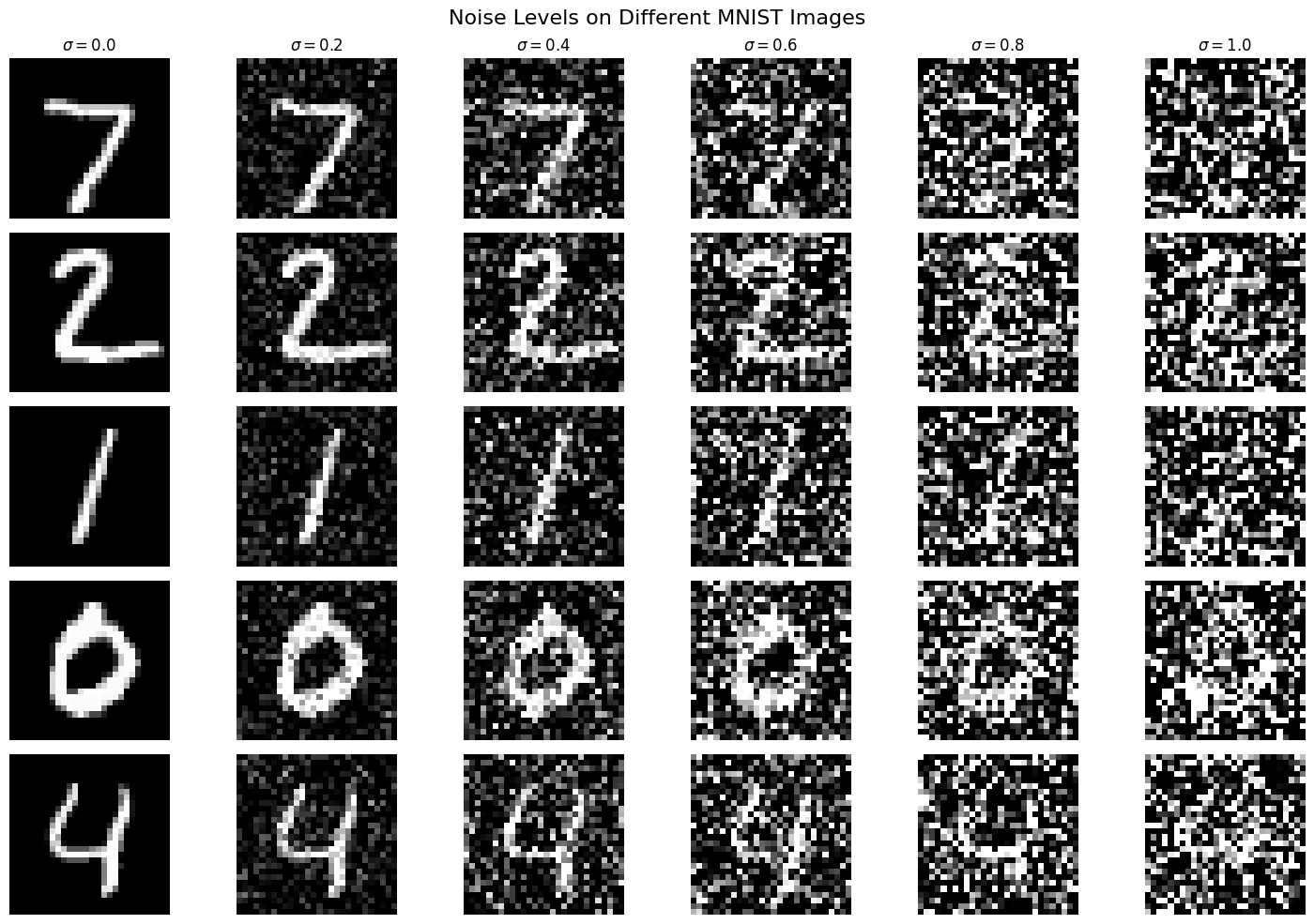
In this part of the project, we trained a U-Net to denoise a noisy MNIST digit. To create the training dataset, we added noise to the MNIST images. Here are some examples of varying noise levels:

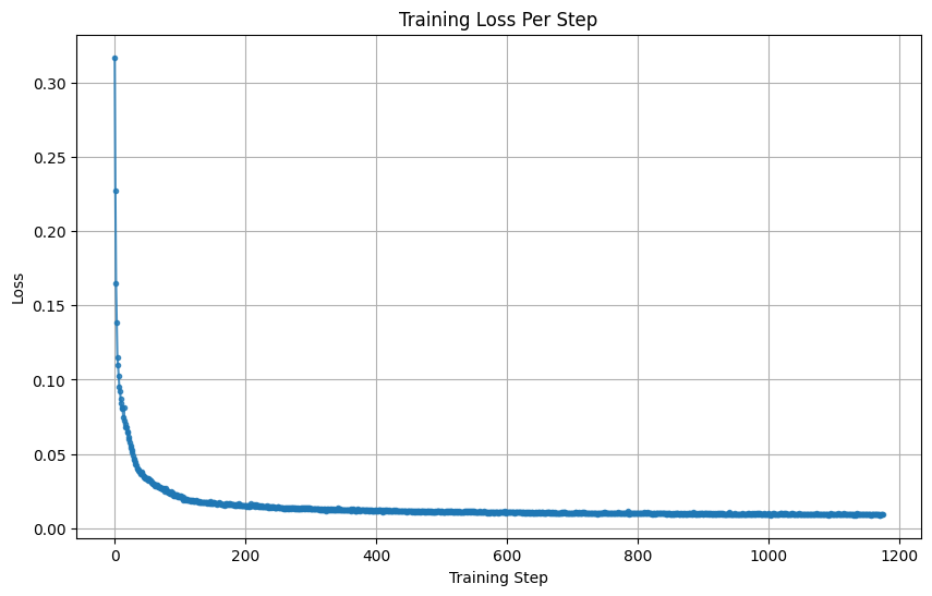
Noise Levels on MNIST Digits — Varying noise levels on MNIST digits.

Here is our training loss over epochs:

Training Loss Graph — Training loss over epochs.

Here are sample results after the first epoch:

Sample Results after Epoch 1 — Sample results after the first epoch.

And here are sample results after the fifth epoch:

Sample Results after Epoch 5 — Sample results after the fifth epoch.

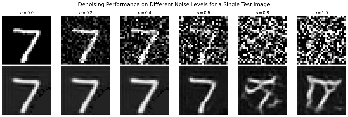
We also ran the model on varying sigma values to observe its performance:

Model Performance on Varying Sigmas — Model performance on varying sigma values.

Part 2: Training a Diffusion Model

Adding Time-Conditioning

We modified our U-Net to predict the noise of an image instead of performing the denoising itself. This approach allows for iterative denoising, which works better than one-step denoising. By adding conditioning on the timestep of the diffusion process, the model understands which step we are at in the iterative denoising process.

To train the model, we took a batch of random images, added noise to each image with a random timestep value from 0 to 299 using the first equation from Part A (0 being no noise and 299 being pure noise), ran the model on the noisy images to get the predicted noise, and then calculated the loss between the predicted noise and the actual noise added.

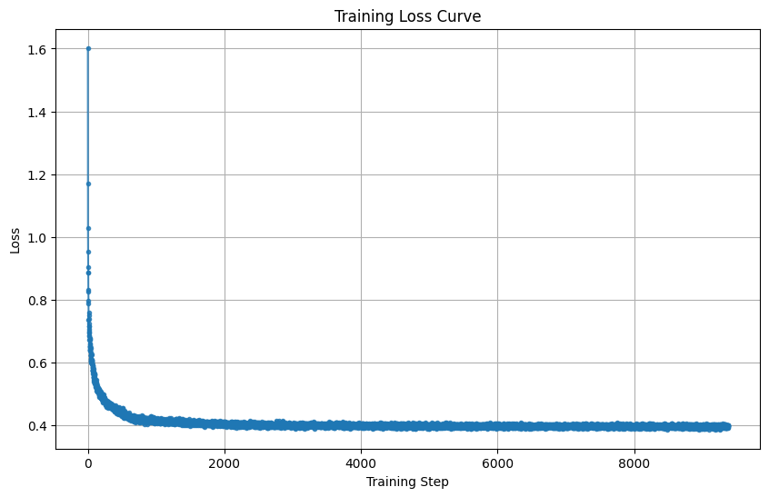
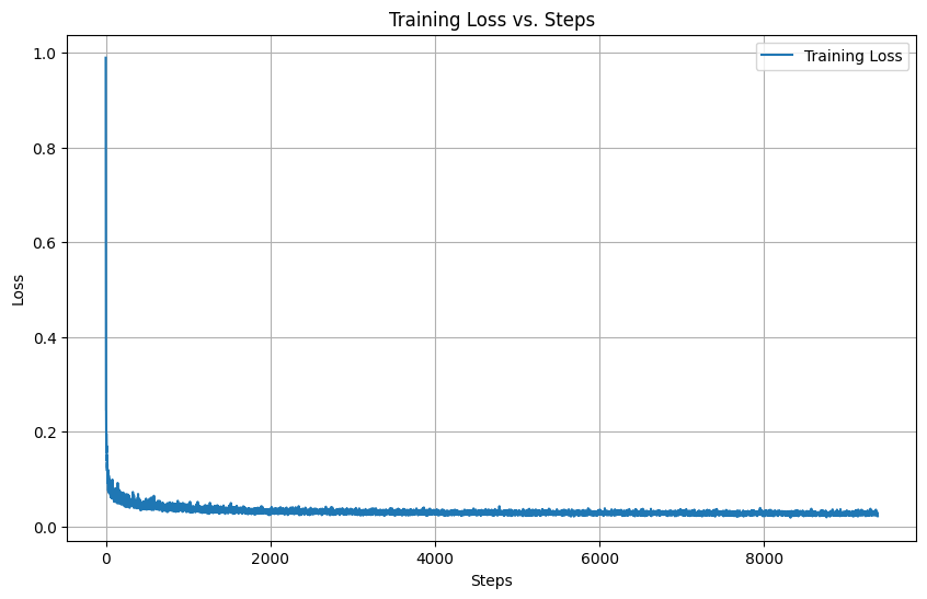
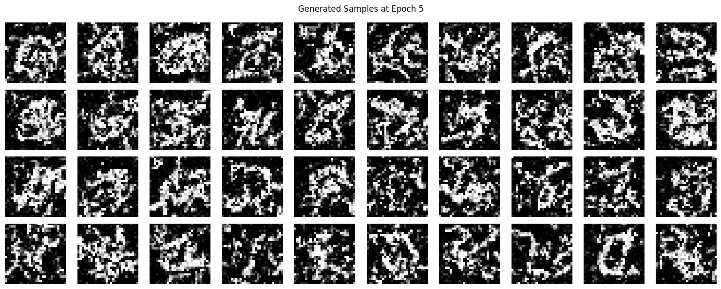
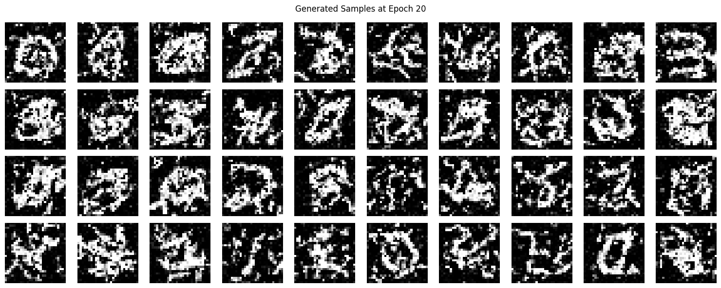
To sample from the model, we ran the iterative denoising algorithm from Part A. Starting from an image of pure noise, we iteratively moved towards the clean image. Since the model was trained equally on all noise levels, it should properly denoise the image after sufficient training. Here is our training loss graph:

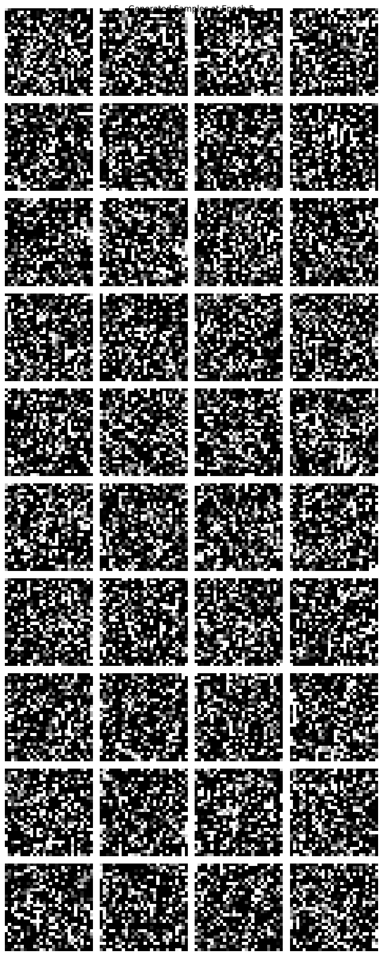
Time-Conditioned Training Loss Graph — Training loss over epochs for time-conditioned U-Net.

Here are the sample results after the fifth epoch:

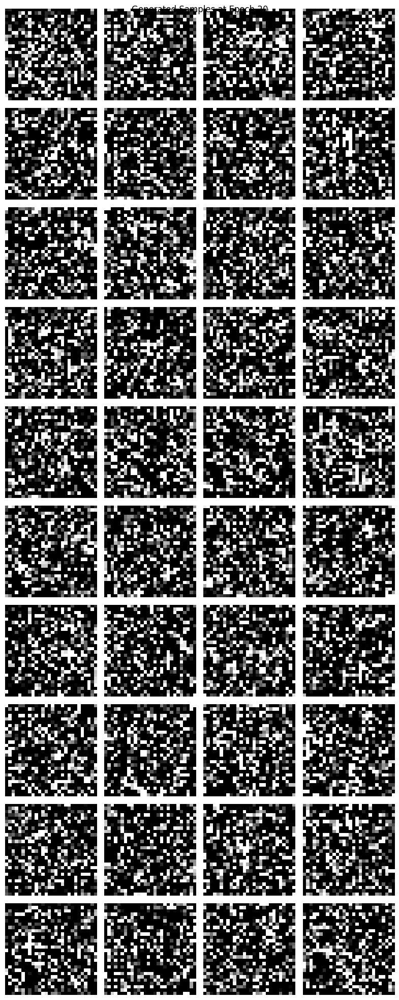
Time-Conditioned U-Net Results after Epoch 5 — Time-Conditioned U-Net Epoch 5 Results.

And here are the sample results after the twentieth epoch:

Time-Conditioned U-Net Results after Epoch 20 — Time-Conditioned U-Net Epoch 20 Results.

Adding Class-Conditioning

In the previous section, the model struggled to generate distinct digits because it lacked the ability to distinguish between different numbers, often producing amalgamations. To address this, we added class-conditioning to our U-Net, providing the specific digit label to guide the generation process.

The training algorithm remained largely the same, but we included the MNIST labels as a "class" vector input to the U-Net. When sampling, we passed in the class vector corresponding to the desired digit. Here are some results from training the class-conditioned U-Net.

Class-Conditioned Training Loss Graph — Training loss over epochs for class-conditioned U-Net.

Class-Conditioned U-Net Results after Epoch 5 — Epoch 5 Results

Class-Conditioned U-Net Results after Epoch 20 — Epoch 20 Results